This is detailed guide to calculating Average True Range (ATR) in Excel. We will first calculate true range and then ATR as moving average of true range. We will cover all three popular ATR calculation methods – simple, exponential, and the original Wilder's smoothing method.
You don't need advanced Excel skills for these calculations – they only use relatively simple Excel functions, such as MAX or AVERAGE.
Historical Data
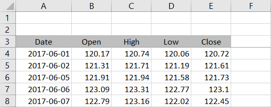
For calculating Average True Range you need the history of high, low and close for each day or bar. If you have your data in OHLC format, paste it into a new Excel spreadsheet into columns A (date/time), B (open – not really needed), C (high), D (low), E (close). Put the column labels in row 3 and the actual data below, starting from row 4.

I will use daily prices for the GLD ETF from 1 June to 31 August 2017. If you want to follow this tutorial with the exact same data and check that your results are correct, you can download the data from Yahoo Finance (the symbol is GLD). Note that I have rounded the prices to two decimal places to deal will Yahoo data imprecision.
You can also calculate ATR for other frequencies, such as weekly, monthly or intraday – the formulas are the same. I will use "day" and "bar" interchangeably to refer to one row throughout this tutorial.
Calculating True Range
Before ATR itself we must first calculate true range for each day, because ATR is a moving average of that. The formula is quite simple – true range is the greatest of the following three price differences:
- High minus low (the traditional range)
- High minus previous close
- Previous close minus low
For detailed explanation and graphical examples, see True Range and How It Differs from Range.
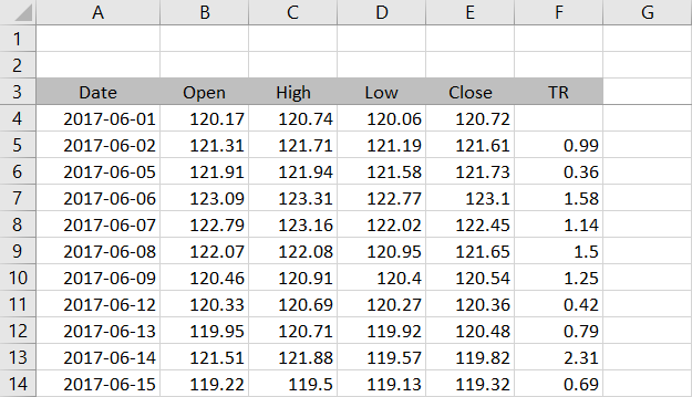
Because the inputs include previous close, we can't calculate true range for the first row of our data, so we will start with the second (row 5 in our spreadsheet). Let's put true range in column F. The formula in cell F5 is:
=MAX(C5-D5,C5-E4,E4-D5)... where C5 is current bar high, D5 is current bar low, and E4 is previous bar close. MAX is the Excel function which returns maximum of given arguments.

Make sure you use relative references (no dollar signs) and copy the formula to the other rows from row 6 down.

We have calculated true range for each bar. Now we can calculate ATR as moving average of true range.
Calculating ATR: Three Methods
There are three popular smoothing methods for calculating ATR from true range. The simple moving average method is the simplest of the three, so we will start with that one. Then we will also calculate the other two methods – exponential moving average and Wilder's smoothing method, which is the original method used by J. Welles Wilder, the inventor of ATR.
Simple Moving Average ATR
The SMA method is very straightforward. In Excel you calculate ATR simply as arithmetic average of true range over a certain number of latest bars, using the Excel function AVERAGE. "Certain number" of bars is called the ATR period and it is the only parameter that this indicator takes.
In this tutorial I will use 21 as the ATR period. I am working with daily data and 21 trading days corresponds to approximately one month. There is no "correct" period and different settings suit different purposes, different markets, and different trading styles.
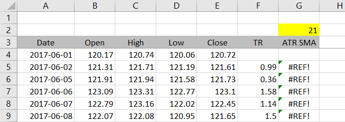
Let's put the period setting in cell G2.

In column G we will calculate the AVERAGE of column F (true range). We will make our calculations dynamic, which will allow as to change the ATR period easily just by changing the value in cell G2, without the need to rewrite any formulas.
We can do this by combining AVERAGE with another Excel function – OFFSET. Let's start in the last row of our data. The formula in cell G68 is:
=AVERAGE(OFFSET(F68,1-G$2,0,G$2,1))
AVERAGE-OFFSET Combination Explained
The entire OFFSET function is inside the AVERAGE function as its argument. OFFSET returns a range of cells and AVERAGE then calculates arithmetic average of those cells.
OFFSET itself has five arguments, which specify the range of cells to return. Let's explain each.
The first argument, "reference", is where you want to start looking for the range. In our example it is cell F68, which is the current bar's true range.
The next two arguments, "rows" and "cols", decide how many rows up or down and how many columns left or right to shift to find the starting point of the range. In our case, we want the range to always include n last rows in column F, ending with F68, where n is the ATR period in cell G2. With the current period setting of 21, we need the "rows" argument of OFFSET to be -20 to shift 20 rows back from cell F68 to cell F48. ATR will be calculated as average of 21 cells from F48 to F68. The "cols" argument is zero, because we want to stay in column F.
The last two arguments, "height" and "width", decide the size of the range. In our case we want "height" to be equal to the ATR period and "width" equal to 1.
You can test the formula by setting a small ATR period like 2 or 3 and checking that it returns arithmetic average of the cells you expect. The result for GLD daily data at 31 August 2017 with ATR period 21 is 1.111905. This is the Average True Range of GLD in the 21 trading days ending 31 August.
You can copy the formula to the other rows to get a time series of ATR.
Fixing the #REF! Errors
In the first few rows you can see that our ATR calculation returns #REF! errors. This is because the formula is trying to calculate AVERAGE of a range that would start before row 1. For example, you can't go 20 rows up from row 5.

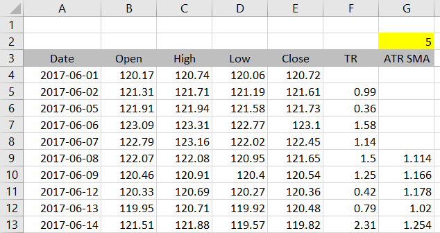
If you don't want to see these errors and prefer empty cells, adjust the formula in cell G5 as follows:
=IF(ROW(F5)>=4+G$2,AVERAGE(OFFSET(F5,1-G$2,0,G$2,1)),"")This is an IF function checking that the row number is high enough for ATR to be calculated. If it is, the formula calculates ATR. If it isn't, the formula returns "". The condition is:
ROW(F5)>=4+G$2If the row number is greater than or equal to 4 plus the ATR period, ATR can be calculated. For example, if you set the ATR period to 2, the first row where ATR calculation is possible is row 6, because the first row of data is 4, the first row with true range is 5, and you need at least two rows with true range, which is 5 and 6.
Note that this formula only works when the first row of data is row 4. If you insert or delete rows and your data starts in another row, you will need to adjust this formula. There are different ways to make this dynamic too – I leave that up to you.
The first rows of our spreadsheet now look like this:

Exponential and Wilder's Method
We have successfully calculated Average True Range using the simple moving average method. For the other two methods, continue to the second part.