This is part 4 of the Binomial Option Pricing Excel Tutorial.
In the previous parts we have prepared our inputs, explained how binomial trees work, and prepared binomial trees in our spreadsheet.
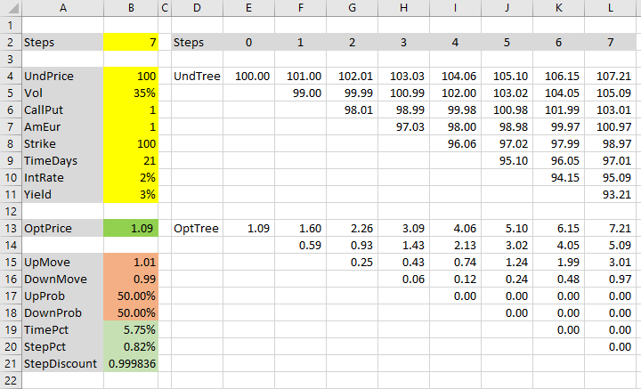
We have used dummy values for up and down move sizes and probabilities. In this part, we will replace them with correct values, calculated according to the Cox-Ross-Rubinstein model.
How Cox-Ross-Rubinstein Model Works
Cox-Ross-Rubinstein (see all formulas and reference) is the best known binomial option pricing model. It is also one of the simplest to calculate.
Its main idea is that up and down move sizes are symmetric. When price moves up one step and then down one step, it returns to its original level. Mathematically:
u · d = 1
... where u and d are up and down move multipliers, which we have in cells B15 (named UpMove) and B16 (DownMove).

Currently these cells contain fixed values. We will replace them with correct formulas.
Calculating Up Move Size
Cox-Ross-Rubinstein move sizes only depend on two things:
- Volatility
- Duration of one step
Volatility σ is one of the model inputs. We have it in cell B5, named Vol.
Duration of one step Δt is time to expiration t divided by number of steps n. We already have it calculated in cell B20, named StepPct (as step percent of year, because the units are years, not days).
The formula for up move multiplier is:

We will replace the fixed value in cell B15 (UpMove) with this formula:
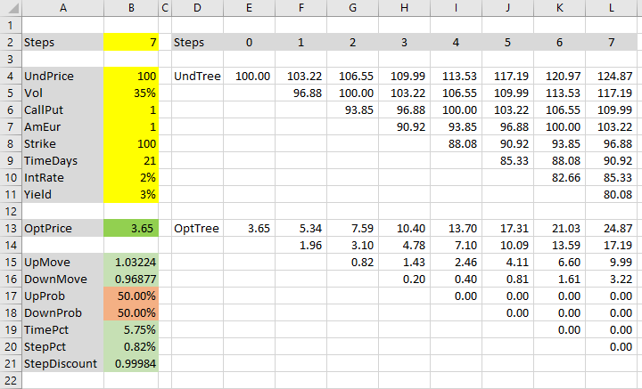
=EXP(Vol*SQRT(StepPct))If you are using the same inputs, you should see 1.03224, which means price increases by 3.2224% in one step up move.
If you see a #NAME! error, make sure you have registered the cell names Vol and StepPct.
Calculating Down Move Size
Calculating down move size (cell B16 named DownMove) is even easier. Because:
u · d = 1
Then:
d = 1 / u
The formula in cell B16 must be:
=1/UpMoveLet's change the background of cells B15 and B16 to green, as they no longer contain temporary dummy values, but correct formulas.

Cox-Ross-Rubinstein Tree Properties
Our underlying price tree (in cells E4-L11) is now correct, according to Cox-Ross-Rubinstein model.
An important characteristic of Cox-Ross-Rubinstein trees is that the same prices keep reoccurring in subsequent steps. Our initial underlying price 100 appears not only in the first cell E4, but also in cells G5, I6, K7 – the middle node in every other step.
The entire underlying price tree is centered around the initial underlying price 100 all the way to expiration.
There is no drift.
Volatility and Drift
In quantitative finance, price movement typically has two components: volatility (how big the moves are in absolute terms) and drift (an upward or downward tendency that makes the price drift to higher or lower levels, on average, over time).
You can think of drift as (very long-term) trend and volatility as noise.
Both these components are contained in our inputs in cells B4-B11.
Volatility is clear – the Vol input, cell B5.
Drift may be less obvious. It is included in two inputs:
- Interest rate (cell B10, which we have named IntRate)
- Yield (cell B11, Yield)
Yield can be continuous dividend yield for stock or index options, or foreign currency interest rate for currency options.
IntRate is always the domestic risk-free interest rate.
In financial formulas, interest rate is typically denoted r and yield q.
Because Cox-Ross-Rubinstein model does not consider r and q in move size formulas, it must consider them in move probabilities.
Calculating Probabilities
Cox-Ross-Rubinstein up move probability formula is:

We already have all the inputs, so we can calculate it in our UpProb cell B17:
=(EXP((IntRate-Yield)*StepPct)-DownMove)/(UpMove-DownMove)DownProb (cell B18) is again very simple, because the two probabilities must add up to 1:
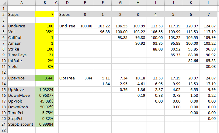
=1-UpProbWith our particular inputs, the probabilities are 49.08% and 50.92%. Let's make cells B17 and B18 green – they contain correct Cox-Ross-Rubinstein formulas now.

Option Price
Both our binomial trees – underlying price tree in cells E4-L11 and option price tree in cells E13-L20 – are correct now, using Cox-Ross-Rubinstein move sizes and probabilities.
The resulting option price can be found in the first cell of the option price tree (E13), or in cell B13, which links to it. With our inputs it is $3.44.
Now you can price different options with the Cox-Ross-Rubinstein model – just change the inputs in the yellow cells B4-B11. The spreadsheet works for American, European, call, put, options on stocks, indexes, or currencies (for currency options, foreign rate goes into the Yield input cell).
If you want to change the number of steps, you need to do two things: change the number in cell B2 and change the actual binomial trees. They must match. You could make the tree calculations change automatically based on the value in cell B2 by adding some IFs to the tree cell formulas (that is beyond the scope of this tutorial; I have done it in the Binomial Option Pricing Calculator).
Next: Jarrow-Rudd Model
The reason why this tutorial creates the trees first, and move size and probability formulas after, is that the former is the same for multiple binomial models. Therefore you can use the first three parts of the tutorial for different models. This is the first model-specific part. In the next parts, you can find move size and probability calculations for Jarrow-Rudd and Leisen-Reimer models.
Continue to Jarrow-Rudd Model in Excel.