This page explains how to calculate historical (realized) volatility from daily closing prices in Excel.
Things Needed for Calculating HV in Excel
- Historical data (daily closing prices of your stock or index) – there are many places on the internet where you can get it for free, such as Yahoo Finance or Alpha Vantage.
- Excel – this guide works for all Excel versions. There is one little difference for versions 2007 and older, which I will point out.
Excel Functions Used
Historical volatility calculation is not that complicated. We will only use the following Excel functions:
- LN = natural logarithm – to calculate daily logarithmic returns
- STDEV.S = sample standard deviation – to calculate standard deviation of these returns
- SQRT = square root – to annualize volatility
Don't worry if you are not familiar with some of them. That's what this page is for. Besides these functions it is only the very basics – multiplication, division, copying formulas etc.
So let's get started. We'll start from scratch – just open a new blank Excel worksheet.
Step 1: Put Historical Data in Spreadsheet
Historical volatility is calculated from daily historical closing prices. Therefore the first step is to put historical prices in our spreadsheet.
In this example I will be calculating historical volatility for Microsoft stock (symbol MSFT), using Yahoo Finance data from 31 August 2015 to 26 August 2016.
If you don't have data, want to use Yahoo Finance and don't know how to find and download data from there, I have created a detailed tutorial (using the same MSFT example).
We will put the data in columns A (date) and B (closing price). Use row 1 for header, so we know which column does what later when we add more columns.
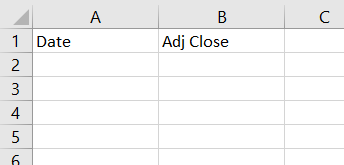
If your stock pays dividends or has history of splits or other actions affecting its price, it is better to use historical closing prices adjusted for these (usually called Adjusted Close), otherwise you will get misleading numbers. This is also what I will do with Microsoft stock.
Paste the data in rows 2 and below.
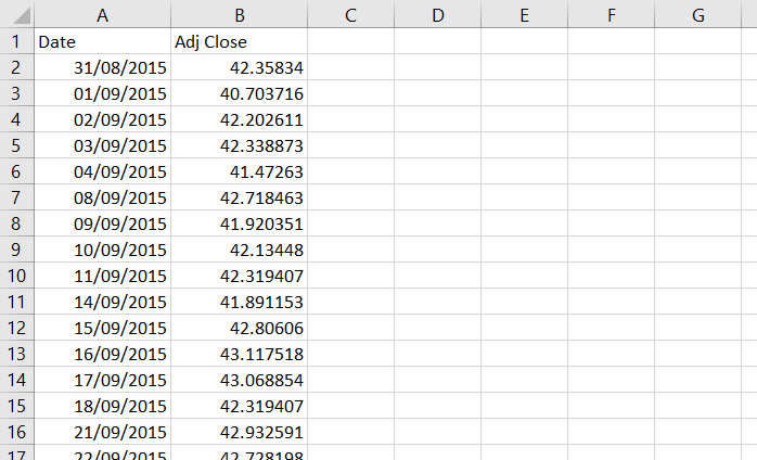
Now you should have historical data ready in columns A and B and you can start the actual historical volatility calculation.
Step 2: Calculate Logarithmic Returns
Historical volatility (at least the most common calculation method which we are using here) is calculated as standard deviation of logarithmic returns. Therefore we first need to calculate these logarithmic returns (also called continuously compounded returns) for every day (row) – we will do this in column C.
It is very simple: daily logarithmic return is the natural logarithm (ln) of the ratio of closing price and the closing price the day before. Mathematically:

In Excel we will use the LN function, which has only one argument – the number x for which we want to find the natural logarithm ln(x). In our case the x is the ratio of closing prices. Therefore, the formula in cell C3 will be:
=LN(B3/B2)where cell B3 is the current day's closing price and cell B2 the previous day's closing price.
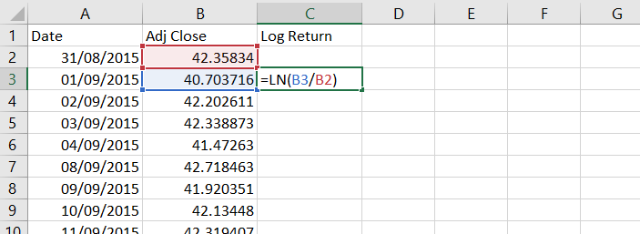
Copy the formula to the rest of column C. The return can't be calculated for the first day, because we don't know the previous day's closing price, so we keep cell C2 empty.
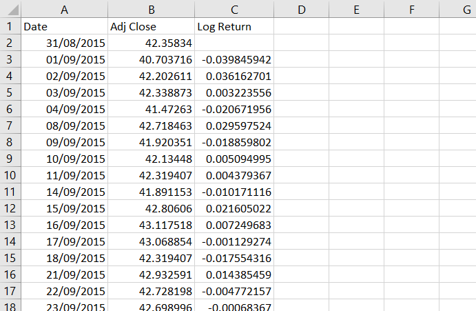
We have now calculated daily logarithmic returns.
Step 3: Calculate Standard Deviation
The next step is to calculate standard deviation of these daily returns.
Standard deviation is the square root of variance, which is the average squared deviation from the mean. I have explained its calculation in detail on this page, but you don't really need to worry about it, because Excel has a built-in function for standard deviation. Actually there are two functions, because there are two kinds of standard deviation: population standard deviation and sample standard deviation. The difference is explained here.
For historical volatility calculation we will use sample standard deviation and the Excel formula for that is STDEV.S (if you are using Excel 2007 or older, the formula is STDEV – without the ".S"; everything else is the same).
This formula takes only one argument and that is the reference to the cells for which we want to calculate standard deviation. It works with as little as two cells or with as much as your computer can handle. We will calculate standard deviation for each day, using a rolling window – a period of n consecutive days ending on the day for which we are calculating the standard deviation.
Which Period Length to Use?
What is n – how many days to include in our rolling window? That is the big decision that you must make when calculating historical volatility. It is often called historical volatility period and it is similarly used with moving averages and other technical analysis indicators.
If you choose a shorter period (small number of days), the resulting historical volatility will more closely reflect the most recent market action, but over time it will fluctuate more (will be more "volatile"). Conversely, if you choose a long period, it will be more stable, but perhaps it might not sufficiently reflect the most recent developments. There is a tradeoff.
If you have no idea, I recommend those I often use myself:
- 21 trading days = 1 calendar month
- 63 days = 3 months
- 252 days = 1 year
Occasionally I might also look at 10-day historical volatility if something interesting is happening in the market, but I wouldn't go lower than that.
So let's use 21 days for our example. We will calculate each standard deviation using the last 21 returns in column C. The first row where we can do this is row 23, where we will use the 21 returns in cells C3 to C23. The standard deviation formula in cell D23 will be:
=STDEV.S(C3:C23)If you are using Excel 2007 or older, the formula will be:
=STDEV(C3:C23)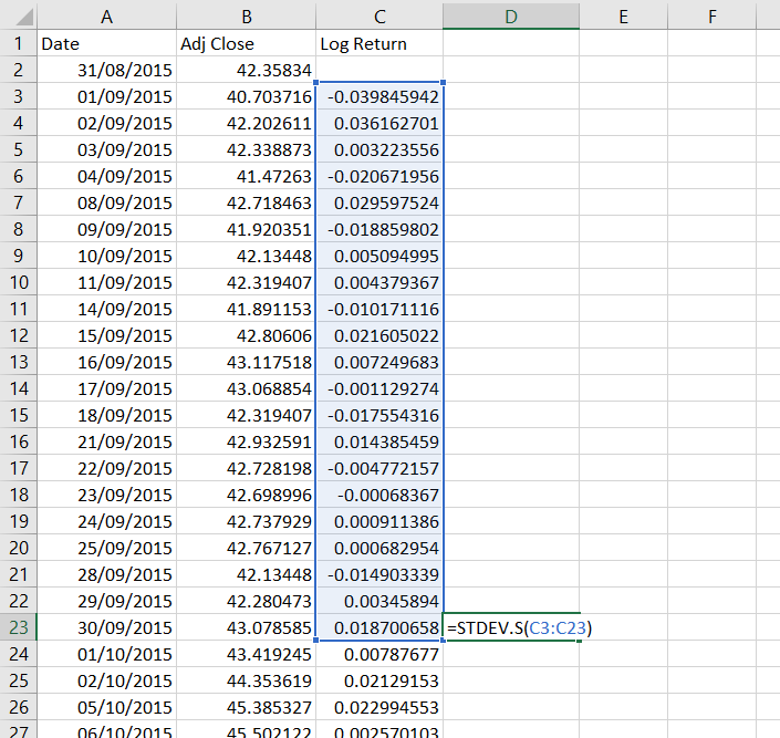
Copy the formula to all other cells below. Cells D2 to D22 remain empty, because we don't have sufficient data to calculate them.
Step 4: Annualize Historical Volatility
Actually, we have already calculated a series of historical volatility values, because that's what the standard deviations are. The only problem is that they represent 1-day historical volatility (because they have been calculated from daily returns). Therefore the final step in our calculation is to convert 1-day volatility to annualized volatility, which is much more common and much more useful.
To convert volatility from daily to annual you need to multiply it by the square root of the number of trading days per year.
Why trading days? Because we have been using a series of trading days (weekends and holidays not included).
Why square root? Because volatility (as we are using it now) is standard deviation and standard deviation is the square root of variance, where the number of days (items) actually enters the calculation. For more detailed explanation see why is volatility proportional to the square root of time.
How many trading days are there in a year? This depends on the market you are working with, as different countries and different exchanges observe different holidays. Furthermore, even for the same country and the same exchange the number of trading days varies from year to year. A good long-term average for US markets is 252 trading days per year, which I will use. If you have longer data history and want to be very precise, you can count the average number of trading days per year directly from your data. But for now let's stick with 252.
We will calculate the annualized historical volatility in column E, which will be equal to column D multiplied by the square root of 252. In Excel, the formula for square root is SQRT and our formula in cell E23 will be:
=D23*SQRT(252)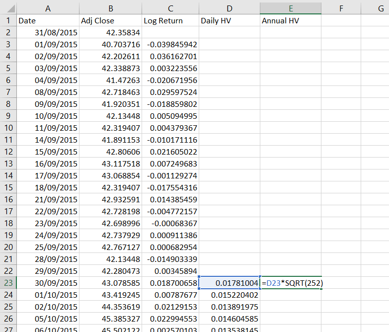
We will again copy this formula to all the other cells below. We can also format columns C, D, E as percentages.
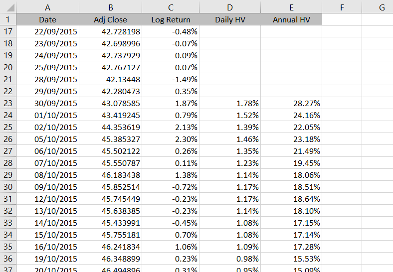
The series we have calculated in column E is historical volatility.
Possible Improvements
There are several ways how we can improve our spreadsheet to make it more useful. In particular:
We can make it support variable historical volatility period length, which the user would enter in some designated cell instead of changing all the standard deviation formulas. Hint: Use the OFFSET Excel function.
We can add a chart. This should be very easy.
You can find these and some more advanced features in the Historical Volatility Calculator.